Using Form Controls in Excel: Combo Box

The Combo Box is used to display a list of items from which only one can be chosen. The list of items to be displayed has to be set up somewhere in the spreadsheet (usually on a separate worksheet) and given a name.

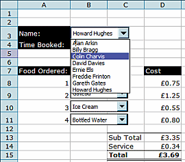
In the image opposite, you can see how the Combo Box appears. It is basically a pull-down list showing the contents of a range of cells. From the Combo Box, one item is selected which then places a value in a previously selected cell. In this example, the third item from the top of the list has been selected, therefore a value of 3 would be entered into the nominated cell.

The value returned from the selected item from the Combo Box can then be used with a variety of other functions to perform operations as required.

Creating the Combo Box
Open a new Excel workbook and in the first worksheet enter a list of 10 names in A1 to A10 (you can make these up or use the names of your favourite football or rugby players!). Once entered, highlight the list of names and give the list a name: Insert>Name>Define... enter people as the name then save the Excel file. Go to worksheet 2 and enter a heading in cell A3 (e.g. Name:). Make sure that the Forms toolbar is open (View>Toolbars>Forms) and select the Combo Box icon. Drag out the Combo Box to the right of the heading in cell A3, then open its Format Control dialogue box (right-click on the combo box). Under the Control Tab, enter people for the Input Range (or use the name you defined earlier), for the Cell Link enter a cell which is off the screen (e.g. N3) and then 5 for the Drop down lines. Click OK to finish the settings, then de-select the Combo Box by clicking on a blank cell. Check that the Combo Box works by clicking its pull-down arrow and selecting a name from the list: also check that a value has been entered into the off screen cell entered into Cell Link above.

Returning information
Once information is selected from a list via a Combo Box, it would be useful if further information could be returned based on the selection. Go back to the worksheet containing the list of names and add two more columns of data: addresses and phone number (fictitious, of course!). Highlight the 3 columns of data and define a name for the area (e.g. pdata) then save the spreadsheet. Return to worksheet 2 and enter the heading Address: in cell A4 (underneath the Name: heading). In cell B4 you are going to use the INDEX function to return the address from the person selected from the Combo Box. 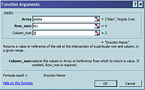The function should look like this:

The Array is pdata - the three columns of data defined as above. The Row Number (Row_num) is the off screen cell which holds the data returned by the Combo Box. Column Number (Column_num) tells the function to return the relevant value from the second column of the pdata area (column 1 holds the names).

After you have completed the Index function, check that it works by selecting different names from the Combo Box, making sure that the correct address is returned. Now perform a similar task by returning the Phone Number data in cell B5.

Extension Tasks
In a new worksheet, create and enter a list of items and prices, for example a restaurant menu, a newsagent or convenience store, a fuel station etc. and use a range of functions to make an invoice page.

Set up a worksheet to record pupils' achievement across a range of subjects. Use the INDEX function on another worksheet to produce individual record sheets.