Checking Conditions - Conditional Formatting

The reason for using Conditional Formatting is to make certain data stand out if it fulfils certain criteria. In this case, if stock levels of book titles fall below a certain level, we can tell Excel to display the information differently, e.g. bold, red text, different colour cell background etc.

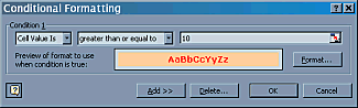To set this up, go to the StockList sheet and highlight all the cells under Current Stock. Select Format from the menu and then Conditional Format... to display the dialogue box. For Condition 1, set the criteria to greater than or equal to from the pull down menu, then enter the value parameter (10 in this case). Now Select the Format... button and choose how you would like the information to be displayed (font style, colour etc.). Finally Select OK when you have set the format. To check that this works, go to the Invoice worksheet and change the Quantity values to between 40 and 50. You should find that the Current Stock values on the Stocklist worksheet have changed according to the parameters you have set.

To make this more useful, you can change the format of the data according to more than 1 condition. In the Conditional Formatting dialogue box, you Add>> more conditions. Set up the formatting so that there are three conditions to be met: one format for when stock is between 11 and 20, one for when stock is between 1 and 10 and a format for when the stock has been depleted. Check everything works correctly before saving the file.

Try setting up Conditional Formatting on the Invoice worksheet to change the format of the In Stock? data depending on its contents.